I was working on a project recently that involved creating images, from one image source, that could come close to mimicking a different image. I was using the OpenCV package, which contains many helpful functions for image processing.
However, one function that I could not find was one for darkening or brightening an image. After writing a function to take care of this for me, I realized that it also offered a good, simple lesson on manipulating arrays with numpy.
All the code, including the final light filtering function, is available here.
You can follow along with this tutorial by checking out the imageFiltering.ipynb notebook provided there. The numpyFunctions.ipynb notebook provides a simpler view of some of the numpy functions used herein.
The file imageFilter.py provides a ready to use function that can apply image filtering to a provide image loaded with OpenCV.

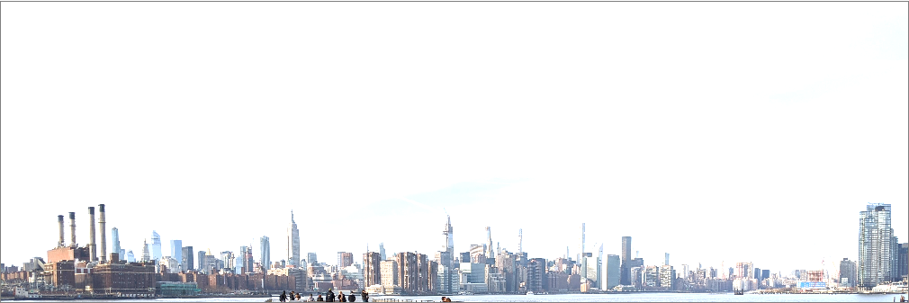
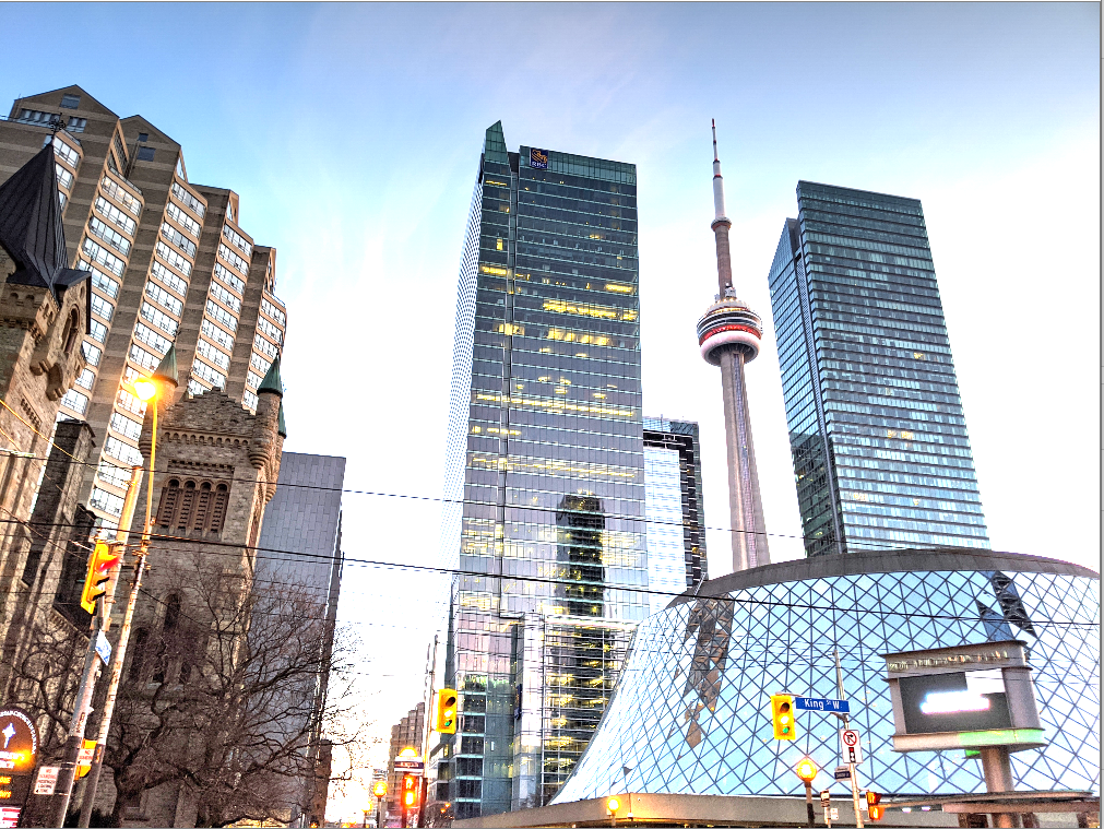
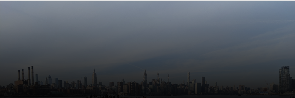
I will be working with two pictures I took with my phone.
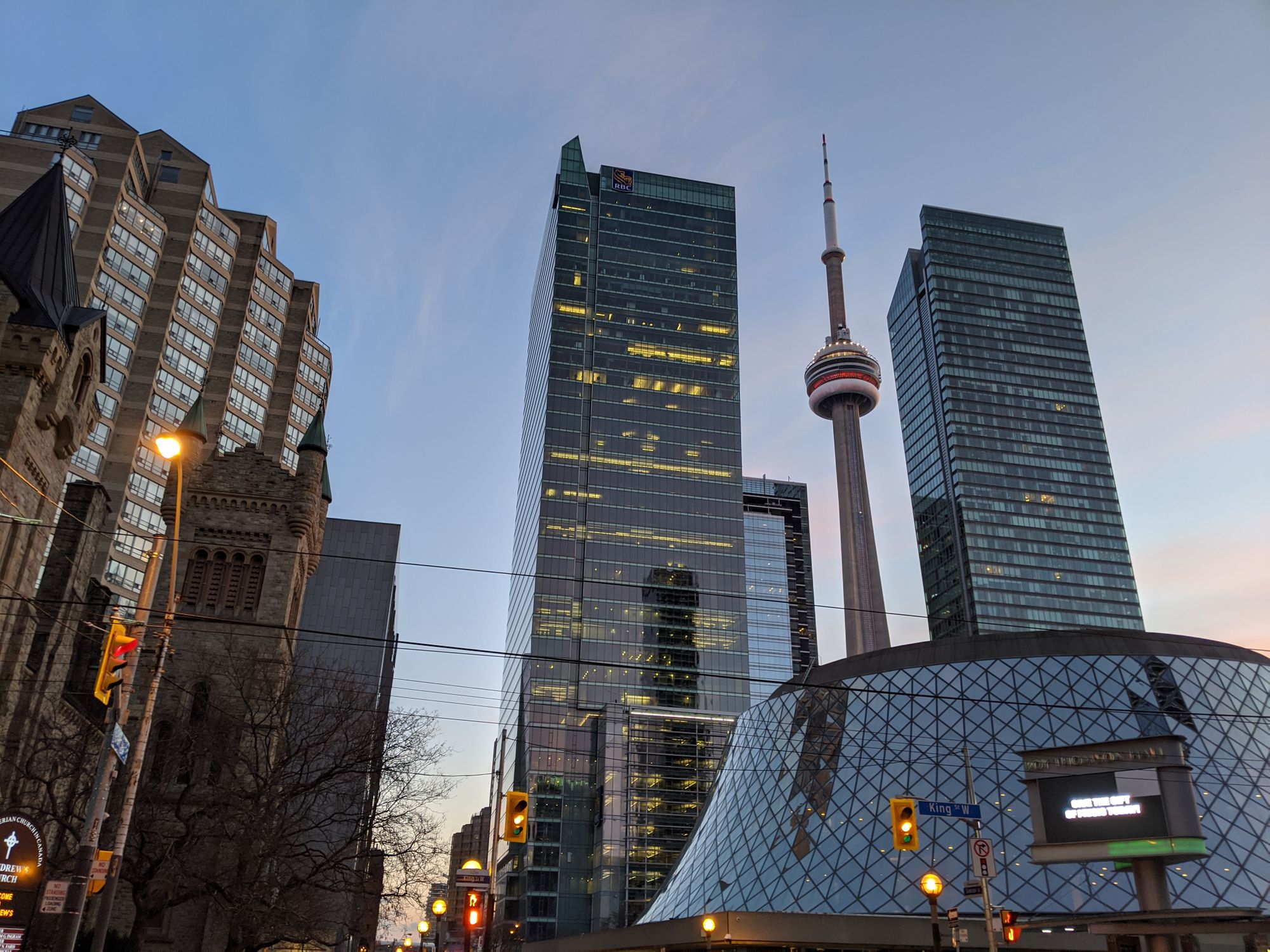
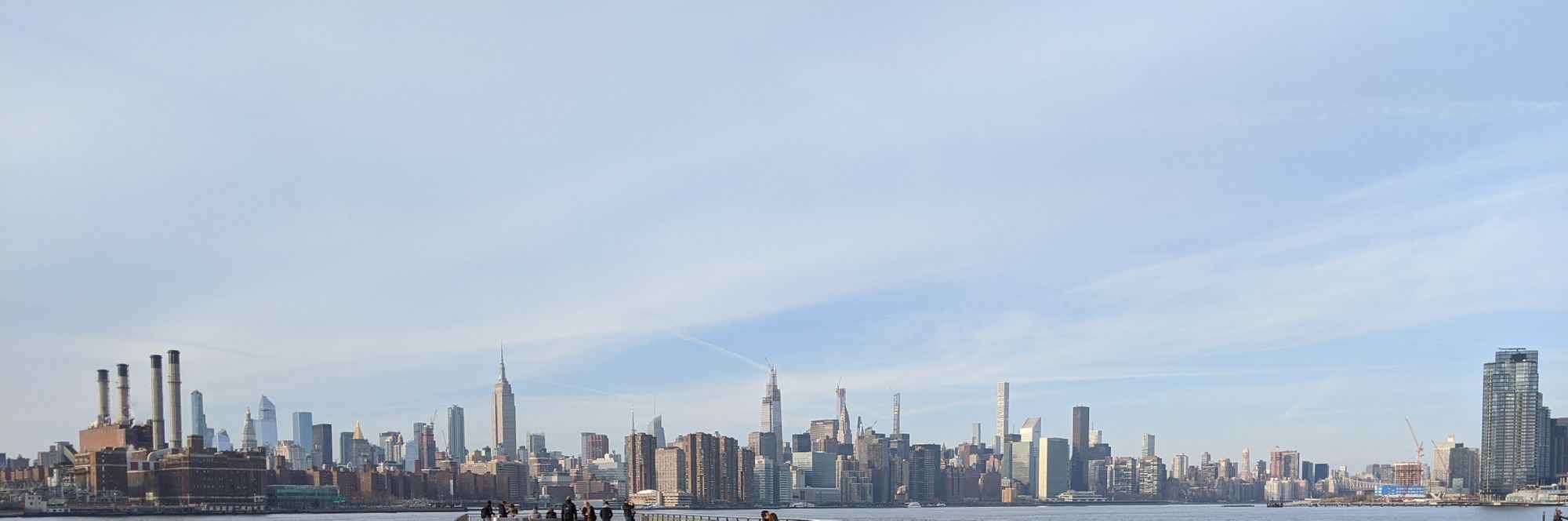
We can import OpenCV and load the images with this function.

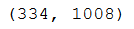
The images, when loaded, are stored as arrays of pixels. We can look at their shape here by calling image_array.shape.
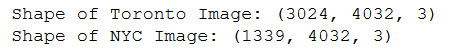
As both are quite large, I will first resize them to 25% of their original size.

Note the dimensions of the array. From the shapes, we can tell the image’s height and width (dimensions 1 and 2 respectively), but what is the third dimension? If you are familiar with a computer’s colour display, this will be a no-brainer – it’s the pixel’s RGB values!
The third dimension is simply the red, green, and blue values. Each one is a number between 0 and 255, and together they give that pixel a specific colouring.
The process of filtering, or lightening/darkening an image, requires only that we increase/decrease these values. For each pixel, we need to do this at the same level for each colour channel.
*Note that you can get access to solid filters like those describe in Part 1 via the Pillow package for Python. If you want to skip this section, go to gradient filtering in Part 2 below.
PART 1 – SOLID FILTERING
If we wanted to apply the same level of brightening across an entire image, we could just update every single pixel with the same percentage, essentially brightening each point by the same amount uniformly. For darkening, it would work the same, but involve a reduction of each pixel’s value instead.
To do so, the first thing we could try is a basic loop. We loop over all 3 dimensions of the array, and update the base elements (the colour channel values), by adding a certain percentage on to them. However, remember that we are constrained by the channel’s themselves. We cannot have a value outside of 0-255. In this case, we can take advantage of Python’s built in min() function, and take the minimum of 255 or our new pixel value.
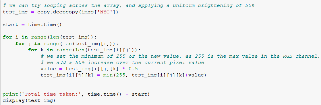

This length of time is fine for just one image. But what if we needed to process hundreds or thousands? That was the problem I faced, as generating thousands of images was already a fairly time-consuming task. Here comes numpy to the rescue!
Since the image we see is stored as a numpy array, we can instead utilize matrix operations to significantly speed up processing time. Specifically, we can use vectorization of a function to apply it across the entire array in a fraction of the original time. While vectorize is actually running loops in the background, it is also running those on compiled C code, which is much quicker than our Python equivalent.
To perform vectorization on our matrix, the first thing we will need is a function. Another handy built-in Python method is the lambda. Lambdas allow us to write quick, one-line functions, and then apply them to our data.

In this case, we are simply creating a function based off our original pixel update.
We can then use numpy's vectorize to make the function applicable to our numpy array.
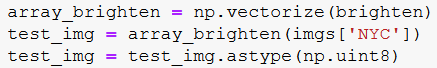
The final result looks like this.


PART 2 – GRADIENT FILTERING
Another way to apply filtering to an image is on a gradient.

Think of a gradient as a gradually changing wave across the image. We can set a starting percentage and ending percentage, and apply a gradient filter that gradually takes the image brighter or darker according to those percentages.
Once again, we can imagine that numpy’s vectorization will help us apply a gradient filtering quickly and easily. We will need to update our method of application however.
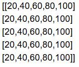
First, let’s consider what we are trying to do. We are trying to apply a gradually changing percentage across an entire array. For example, we would start at 20% at the leftmost column, and slowly up the percentage until we hit 100% at the rightmost column. Each RGB pixel in the column is updated by the same amount, but the next column should be updated by a higher percentage. Here’s what that might look like.
The next thing to consider is how we can apply this array with the original image array. Obviously, we will want to generate this percentage array to be the same size as the image. However, we will not need the third dimension to be of size 3, we can apply the same percentage value across each colour channel.
As it turns out, vectorizing can take in a function that requires two different matrices, and apply the values from one towards updating the other. This means we can use lambda with np.vectorize again, we will just need a slightly updated version.

The last thing we need to figure out is the creation of our percentage matrix. Luckily, numpy still has us covered.
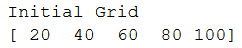
First, we can create our incremental percentages with the function MGrid. This function takes in a low number, a high number, and an increment value, and then increments between the two (the top value is exclusive, while the bottom is inclusive).

Now, we need to consider how we will use this array of numbers. If we repeat the same array downwards, the gradient will move from left-to-right. If we turn the array into a column, and repeat it to the side, we will have a set of percentages changing from top-to-bottom.
To repeat this grid downwards, and create the left-right gradient, we can use np.stack. This function takes in a tuple of arrays to stack, so we will create a tuple with our array repeated n times, and pass it to stack.
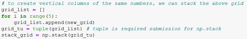
Next, we transpose the stack to set it back on the correct axis.
Finally, we will need to resize this matrix, to make it broadcastable with our 3-D image array. We add a third dimension of size 1.

We can now run our vectorized lambda, passing image and the new array, to reveal the gradient brightness effect.
If we wanted to instead have our gradient on the vertical axis, we can use a slightly different method. Once again, we will use np.mgrid to create the percentage array. However, instead of using np.stack, we can instead use np.tile to expand this array in the proper direction. Tile repeats the given array by a given amount of times. We will transpose the result to give us our vertical axis gradient.

Finally, all we need to do here is reshape the matrix to add our third dimension, with size 1.
We run on our vectorized lambda in the same way as above.
It’s fairly simple to transform the gradient direction as well – the simplest method is to just switch our high and low image values.
The function I provided in imageFilter.py allows you to set the gradient direction as a parameter, rather than just having these values switched.